Exploring cluster stability selection results

The getting-started guide (the package home page) shows how to run cluster stability selection with css(). This vignette shows how to explore and visualize a fitted cssr object using its S3 methods: plot(), print(), summary(), and selected(). All of them read the already-computed selection proportions, so they are cheap to call and let you explore different cutoffs without re-running the (relatively expensive) subsampling.

library(cssr)
set.seed(983219)

# Data with a cluster of 10 correlated proxies for a latent variable (features
# 1-10), plus some unclustered "weak signal" features and noise.
data <- genClusteredData(n = 80, p = 30, cluster_size = 10,
                         k_unclustered = 5, snr = 3)
X <- data$X
y <- data$y

# css() needs a lambda; getLassoLambda() picks one by cross-validation.
lambda <- getLassoLambda(X, y)

# Run cluster stability selection, telling css about the cluster of proxies.
css_output <- css(X, y, lambda, clusters = list("Z_cluster" = 1:10))

Visualizing selection proportions with `plot()`

plot() draws a sorted bar plot of the cluster selection proportions – the proportion of subsamples in which each cluster was selected. The clusters selected at the given cutoff are highlighted, and the cutoff is drawn as a dashed reference line.

plot(css_output, cutoff = 0.9)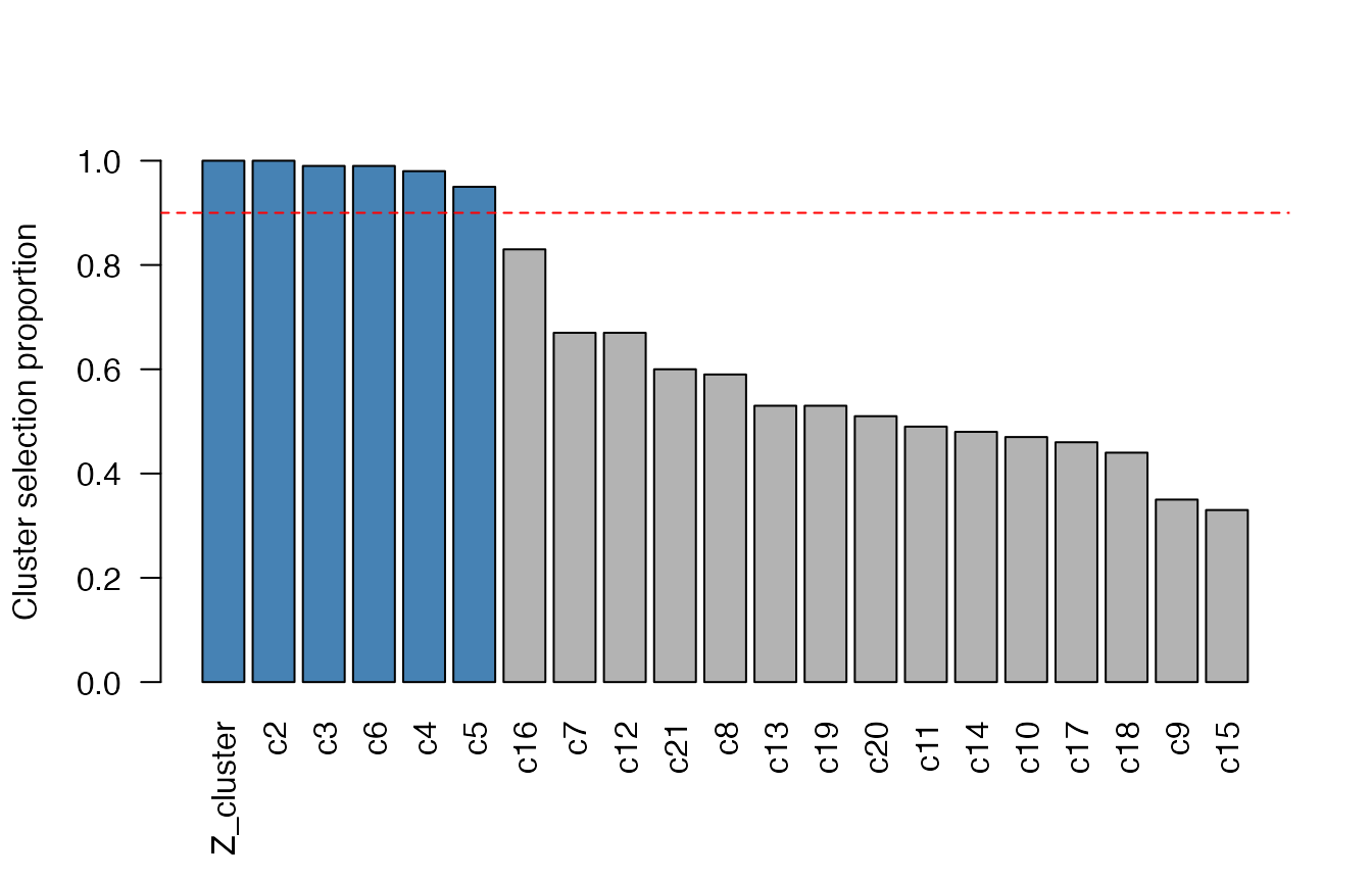

"Z_cluster" (the cluster of proxies) rises to the top – exactly the vote-splitting fix that cluster stability selection provides. Pass type = "features" to plot the individual-feature selection proportions instead:

plot(css_output, type = "features", cutoff = 0.9)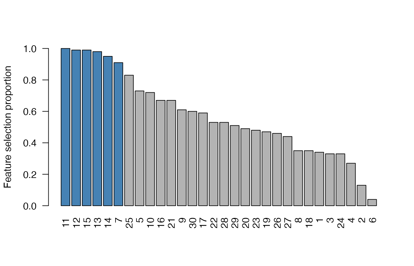

Tabular summaries: `print()` and `summary()`

Printing a cssr object shows one row per cluster, in decreasing order of selection proportion, with each cluster’s prototype (its highest-selected member) and size:

print(css_output, cutoff = 0.9)
#>   ClustName ClustProtoNum ClustSelProp ClustSize
#> 1 Z_cluster             7         1.00        10
#> 2        c2            11         1.00         1
#> 3        c3            12         0.99         1
#> 4        c6            15         0.99         1
#> 5        c4            13         0.98         1
#> 6        c5            14         0.95         1

summary() returns a computable overview (the selection counts plus the per-cluster table) with its own print method:

summary(css_output, cutoff = 0.9)
#> Cluster stability selection summary
#> 6 clusters / 6 features selected at cutoff 0.9
#> 
#>   ClustName ClustProtoNum ClustSelProp ClustSize
#> 1 Z_cluster             7         1.00        10
#> 2        c2            11         1.00         1
#> 3        c3            12         0.99         1
#> 4        c6            15         0.99         1
#> 5        c4            13         0.98         1
#> 6        c5            14         0.95         1
#> 
#> PFER: NA (not yet implemented; see issue #87)

Extracting the selection with `selected()`

selected() returns the selected clusters directly – a named list giving the feature indices in each. Pass type = "features" for the flat vector of all selected features:

selected(css_output, cutoff = 0.9)
#> $Z_cluster
#>  [1]  1  2  3  4  5  6  7  8  9 10
#> 
#> $c2
#> [1] 11
#> 
#> $c3
#> [1] 12
#> 
#> $c4
#> [1] 13
#> 
#> $c5
#> [1] 14
#> 
#> $c6
#> [1] 15

selected(css_output, type = "features", cutoff = 0.9)
#> [1]  7 11 12 13 14 15

plot(), print(), summary(), and selected() all share the same cutoff / min_num_clusts / max_num_clusts arguments, so you can dial the selection in without re-running css().

Visualizing selection proportions with plot()

Tabular summaries: print() and summary()

Extracting the selection with selected()

See also

Visualizing selection proportions with `plot()`

Tabular summaries: `print()` and `summary()`

Extracting the selection with `selected()`